Continuous-Time Fourier Transforms
Representation Theory An important concept from signal processing is that we can often uniquely and completely represent a signal as a weighted […]
Representation Theory An important concept from signal processing is that we can often uniquely and completely represent a signal as a weighted […]
Convolution and Difference Equations We previously demonstrated that the output of any linear, time-invariant system can be expressed by a convolution of […]
The Sifting or Sampling Property At first glance, this may seem like an exercise in tautology. However, this property is key to […]
Representing data as a vector In signal processing, data science, and machine learning, it is ubiquitous to represent quantitative data as a […]
Motivation Throughout the course, we will visualize systems using block diagrams, such as the one shown here. Block diagrams are a straightforward […]
Motivation To analyze and process signals, we must first understand their basic properties: what types of signals exist, how we can measure […]
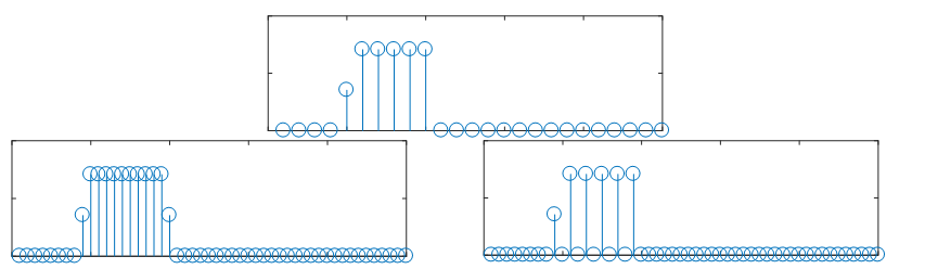
If you’ve ever fiddled with the playback speed on a YouTube video or compressed an audio file to save space, you’ve seen the effects of downsampling and upsampling in action. But here’s the thing: changing a signal’s sampling rate isn’t just about time or file size.
In digital signal processing (DSP), downsampling and upsampling are fundamental building blocks—not just for compression or rate conversion, but for reshaping the way we filter and analyze signals. They’re mathematical lenses that let us zoom into or abstract away different parts of a system.
So yes, shrinking and stretching signals is cool. But if you think that’s all they do, you’re missing the bigger picture.
Let’s face it: most students encounter filters in their first digital signal processing (DSP) course as theoretical constructs—lines of equations, plots of magnitude response, and vaguely threatening phase diagrams.
But in practice, filter design is one of the most critical tasks in digital signal processing, and the decisions you make—FIR or IIR? Windowing or bilinear transform?—can shape whether your application sounds smooth, runs fast, or falls apart in a haze of numerical instability.
This article is your signal-processing decoder ring. We’ll walk through the why and how of FIR and IIR filter design, demystify common design techniques like windowing and the bilinear transform, and help you build intuition for choosing the right method—not just for an exam, but for the real world.
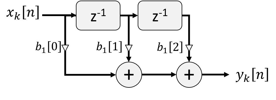
If you’re knee-deep in a graduate-level digital signal processing (DSP) course, you’ve probably designed a filter or two. You’ve plotted poles and zeros, wrangled a transfer function, maybe even written some MATLAB to test a low-pass filter on a noisy signal.
Then someone tells you:
“Great filter. Now pick your structure.”
Wait—what?
Isn’t a filter defined by its difference equation or transfer function? Isn’t that enough?
Short answer: no.
The long answer is what this article is about. Because when you move from the page to the real world—whether it’s a microcontroller, a medical device, or a machine learning pipeline—how you implement a filter matters just as much as what the filter does.
We tend to treat algorithms as transient tools—clever bits of logic that solve specific problems and then fade into the background. But the Fast Fourier Transform, or FFT, is not that kind of algorithm.
The FFT isn’t just a fast way to compute a Fourier transform. It’s a cornerstone of digital signal processing, and by extension, of modern computation. It’s the engine beneath your voice assistant’s signal chain, the speed behind your MRI scanner’s image reconstruction, and the unsung hero of everything from wireless communication to deep learning.
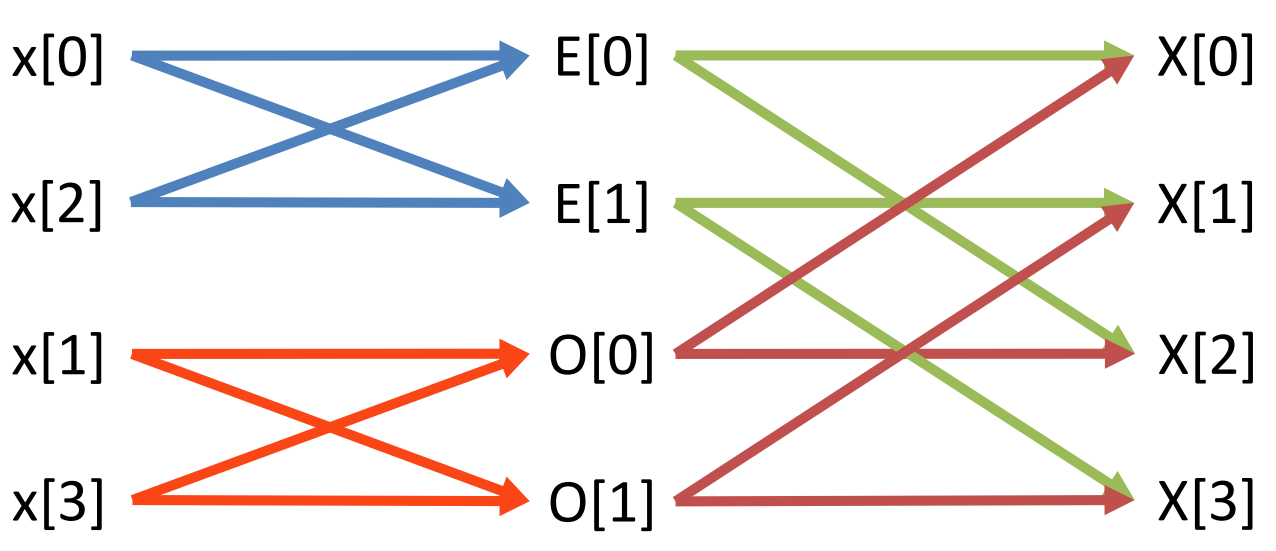
Yet for many, the FFT begins and ends with a textbook diagram of a radix-2 butterfly. That’s a shame, because the FFT is both deeper and more diverse than its most famous form.
Let’s explore what the FFT really is, how it goes beyond radix-2, and why it remains one of the most influential ideas in the applied mathematical sciences.