Convolution and Difference Equations
We previously demonstrated that the output of any linear, time-invariant system can be expressed by a convolution of an input and system impulse response. Here, we show that convolutions can be expressed with differences equations. Hence, any linear, time-invariant system can be expressed by difference equations.
The Difference Equation Form of Convolution
If we use the commutativity property ( ), we see that the convolution can be written as


 are all constant values, the expression above is a difference equation.
Impulse Response Properties
Using our new definition, we can we can derive relationship between our impulse response  and system properties.
Memoryless
An LTI system with impulse response is memoryless if

 .
Causal / Anti-Causal
An LTI system with impulse response is causal if

An LTI system with impulse response is anti-causal if 
A causal system must be dependent on only past and present values. As a difference equation, this can be written as

Hence, this is equivalent to stating  for all
 :

BIBO Stable
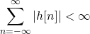
An LTI system with impulse response is BIBO stable if
Finite / Infinite Impulse Responses
FIR Filters
If the impulse response is finite in length (i.e., the number of non-zero values is finite), then the number of terms in the difference equation is finite. We refer to these types of linear, time-invariant systems as finite impulse response filters.
IIR Filters
If the impulse response is infinite in length, the linear, time-invariant systems is a infinite impulse response filter.
Relative to the difference equation, the impulse response may be infinite to two reasons.
The number of difference equation terms is infinite.
The difference equation has recursion (i.e.,  is a function of
 for any
 )
When we have recursive terms, the difference equation can be written as


Graphically understanding difference equations
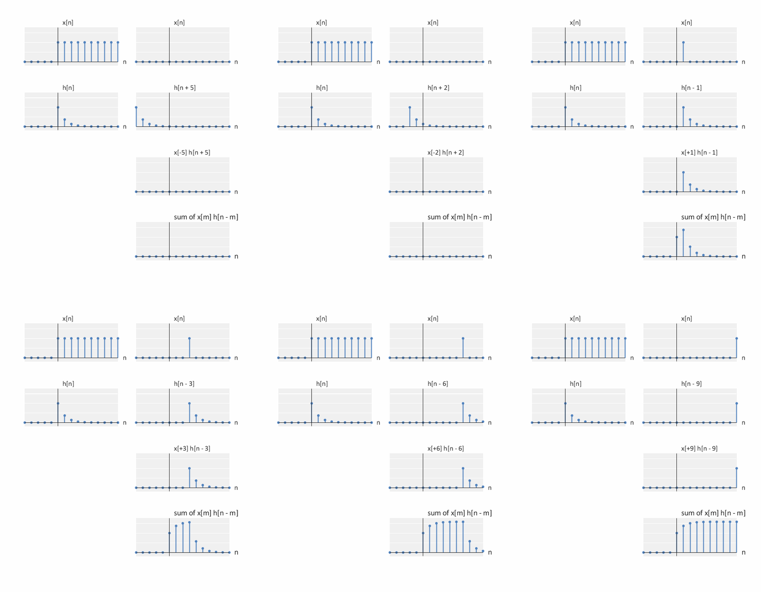
Convolution can be seen as a graphical process:
Plot  with dependent variable
 (
 shifts the signal).
Plot with dependent variable .
For each shift, compute  . These are just weighted version of .
Sum your elements to get  .
Graphical Difference Equation Examples
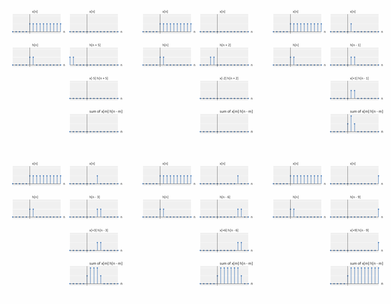
Below are a collection of graphical examples of discrete-time convolution / difference equation solutions.
Box and an impulse


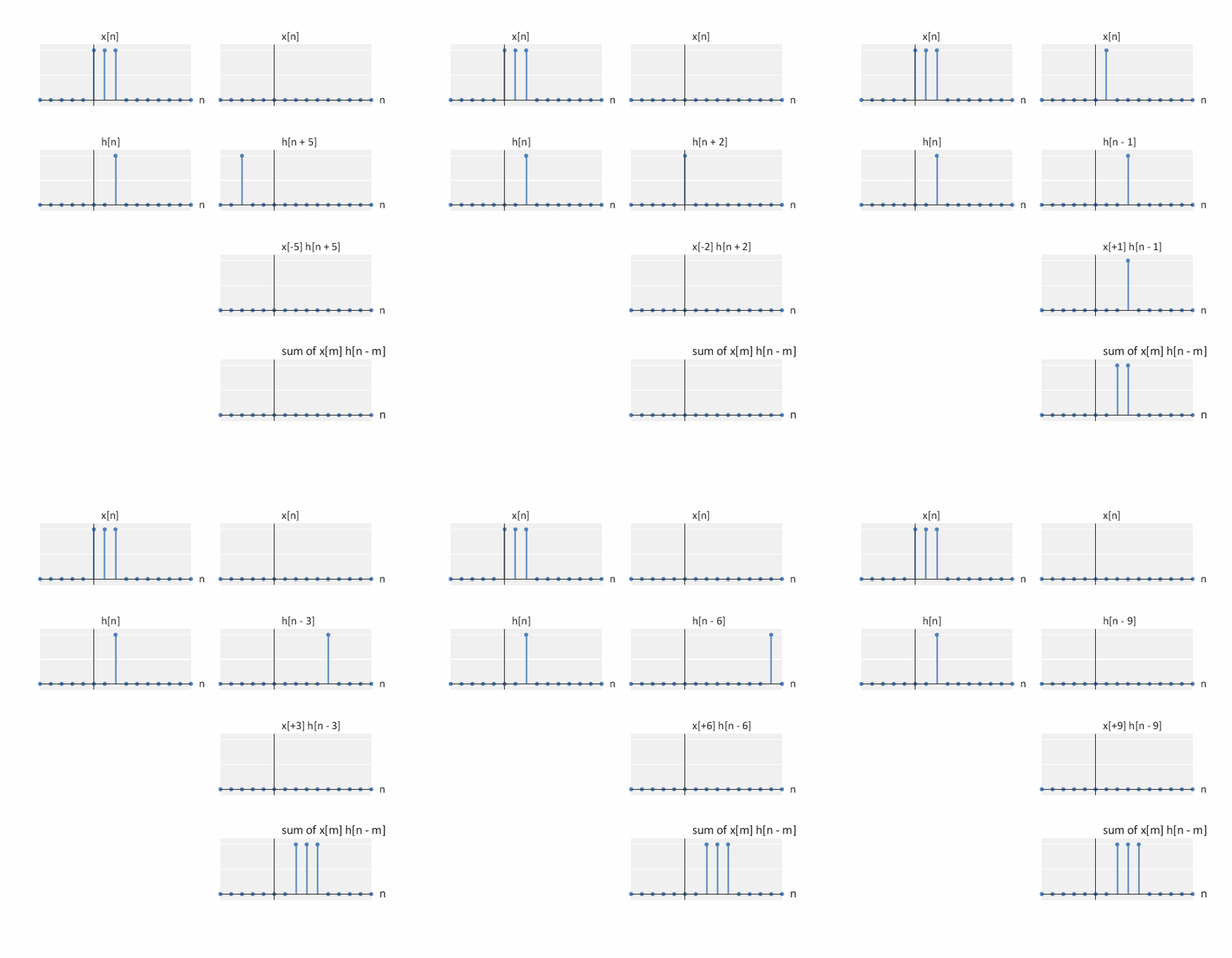
Two boxes

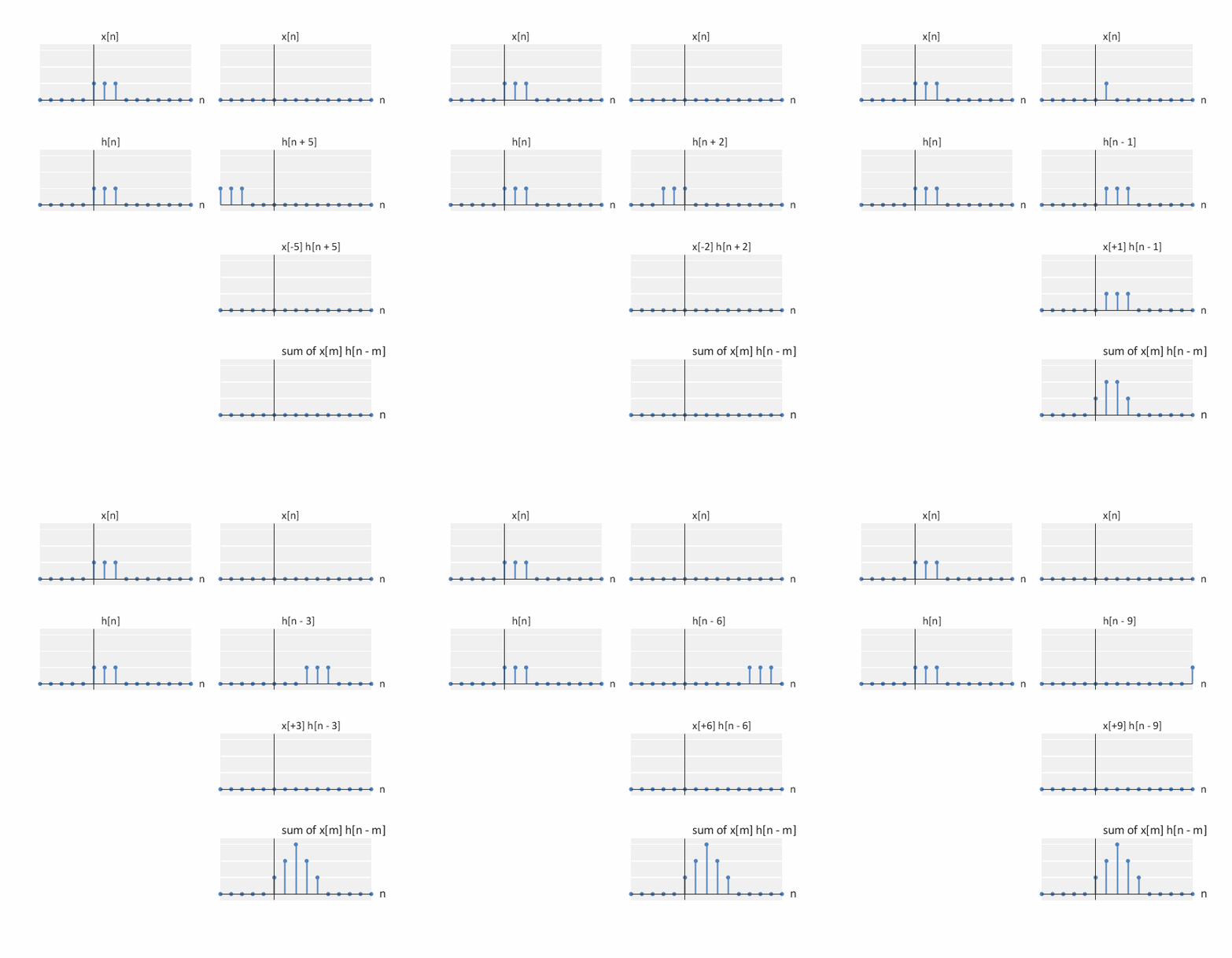
Box and exponential

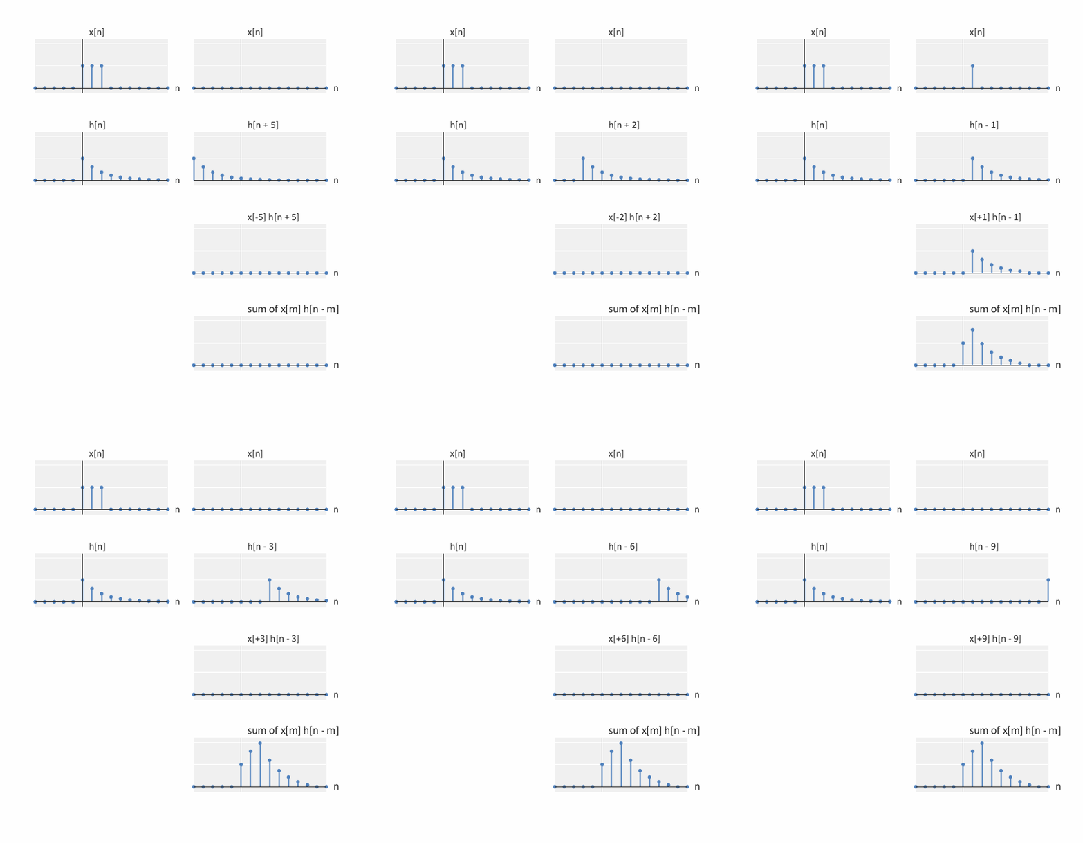
Two exponentials

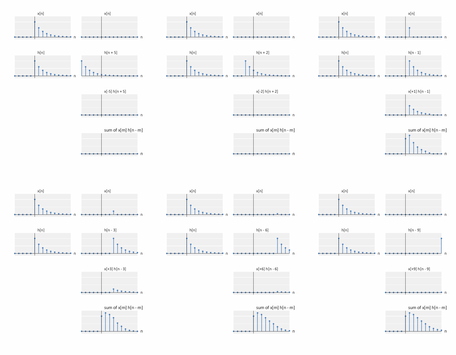
Finite Ramp and Box

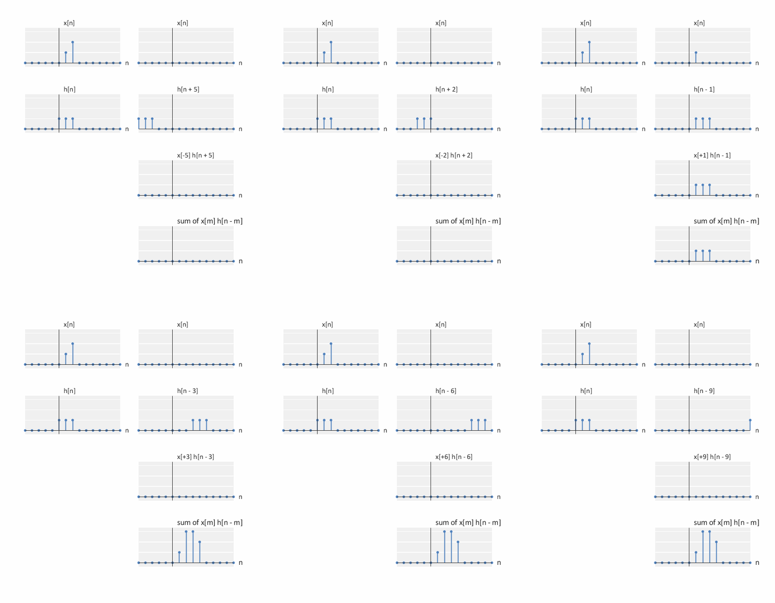
Random Numbers and Box
 random signal
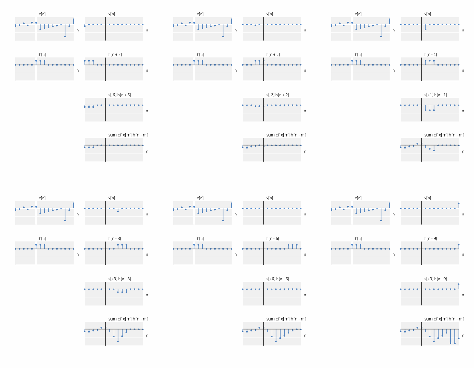
Step function and an exponential

Step function and a box