Sampling

Sampling: Continuous-to-discrete

What is Sampling?

Sampling is the process of converting a continuous-time signal into a discrete time signal.

Sampling is accomplished by multiplying a continuous-time signal x(t) with an impulse train, a periodic sequence of impulses with a fundamental period T_s such that

    \[\delta_{T_s}(t) = \sum_{k=-\infty}^{\infty} \delta(t - k T_s) \; .\]

We will use the notation \delta_{T_s}(t) to represent a pulse train with sampling period T_s. When we multiply x(t) and \delta_{T_s}(t), we get an new train of impulses with amplitudes taken from x(t). Mathematically, we get

    \[x_s(t) = x(t) \delta_{T_s}(t) = \sum_{k=-\infty}^{\infty} x(k T_s) \delta(t - k T_s) \; .\]

The question address in the rest of this class is: does the sampling process uniquely preserve all information about our signal?

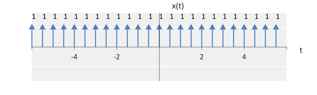
Pulse train in time with Ts=1/2.
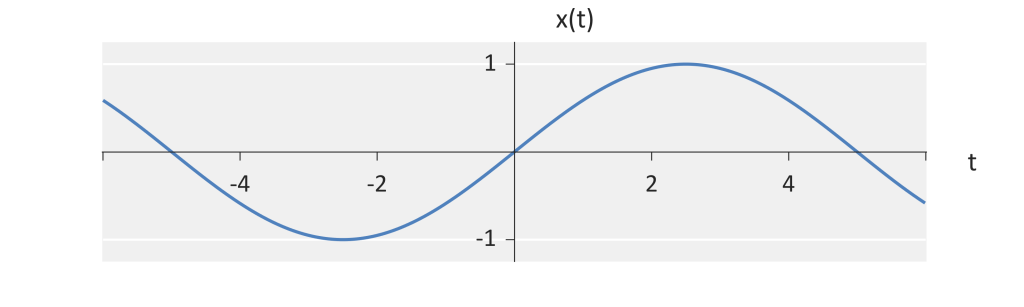
Sinusoid with a period of 10.
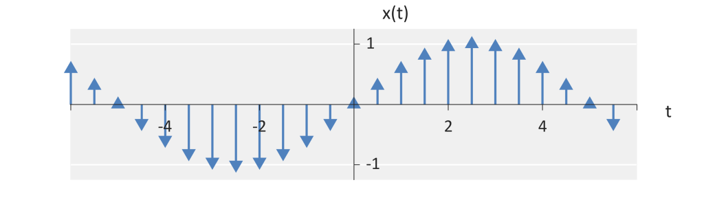
Sampled sinusoid with sampling period of Ts=1.

Fourier Series/Transform of an impulse train

To answer this question, we look at the Fourier series/transform of the impulse train. Since \delta_{T_s}(t) is periodic, we use the Fourier series. When we plug \delta_{T_s}(t) into the Fourier analysis equation, we get

    \[c_k = \frac{1}{T_s} \int_{T_s} \delta_{T_s}(t) e^{-j k \Omega_s t} dt \; .\]

Over one period, \delta_{T_s}(t) is just an impulse. Therefore, the Fourier analysis equation simplifies to

    \begin{align*} c_k &=& \frac{1}{T_s} \int_{-T_s/2}^{T_s/2} \delta(t) e^{-j k \Omega_s t} dt \\ &=& \frac{1}{T_s} (1) \end{align*}

We refer to \Omega_s = 2 \pi / T_s as the [angular] sampling frequency.

Since the Fourier series coefficients are defined by c_k = \frac{1}{T_s}, the Fourier transform has a value of 2 \pi / T_{s} (the 2 \pi is introduced because we are in the angular frequency domain) at k times the fundamental angular frequency, i.e. k \Omega_s = k 2 \pi / T_s, where k is an any integer. Therefore, in the continuous-frequency, we get a pulse train with spacing of \Omega_s,

    \begin{align*} \delta_{T_s}(t) &\stackrel{\mathcal{F}}{\longleftrightarrow}& \frac{2 \pi}{T_s} \delta_{\Omega_s}(\Omega) \\ \end{align*}

Therefore, the Fourier transform of an infinite pulse train with period T_s (i.e., \delta_{T_s}(t)) is a infinite pulse train with spacing \Omega_s = 2 \pi / T_s (i.e., ({2 \pi}/{T_s}) \delta_{\Omega_s}(\Omega)).

Pulse train in time with Ts=1/2.
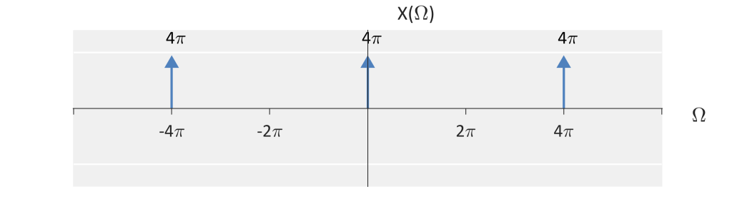
Fourier transform of the above pulse train.

Apply multiplication property

To determine the Fourier transform of x(t) \delta_{T_s}(t), we apply the multiplication property. That is, multiplication in time is equivalent to convolution in frequency. We get the relationship

    \begin{align*} x(t) \delta_{T_s}(t) &\stackrel{\mathcal{F}}{\longleftrightarrow}& \frac{1}{2 \pi} \left[ X(\Omega) * \left( \frac{2 \pi}{T_s} \delta_{\Omega_s}(\Omega) \right) \right] \\ x(t) \delta_{T_s}(t) &\stackrel{\mathcal{F}}{\longleftrightarrow}& \frac{1}{T_s} \sum_{k=-\infty}^{\infty} X(\Omega - k \Omega_s) \end{align*}

Therefore, sampling in time results in the sum of shifted replicas of the frequency domain representation X(\Omega).

A Gaussian pulse signal.
The Fourier transform of the above Gaussian pulse.
A sampled Gaussian pulse signal with sampling period of Ts=1/2 and sampling rate of Ωs=4π.
The Fourier transform the sampled Gaussian pulse with a sampling rate of Ωs=4π.

The sampling theorem

We can now answer our question, does the sampling process uniquely preserve all information about our signal? The answer is: yes, but under certain conditions.

Let the Fourier transform of x(t) be X(\Omega) with a largest angular frequency \Omega_{max}. That is

    \[X(\Omega) = 0 \quad \textrm{for} \quad |\Omega| > \Omega_{max} \; .\]

Also, let X_{s}(\Omega) be defined as the Fourier transform of the sampled signal x_s(t) = x(t) \delta_{T_s}(t) such that

    \[X_{s}(\Omega) = \frac{1}{T_s} \sum_{k=-\infty}^{\infty} X(\Omega - k \Omega_s) \; .\]

If the bandwidth of the X(\Omega), X(\Omega-\Omega_s), and X(\Omega+\Omega_s) never overlap, then the original frequency information is remains changed. That is, to preserve all information about the original signal, we require

    \[\Omega_s > 2 \Omega_{max}\]

or, equivalently,

    \begin{align*} f_s &>& 2 f_{max} \\ T_s &<& \frac{1}{2 f_{max}} \\ T_s &<& \frac{\pi}{\Omega_{max}} \end{align*}

Therefore, the sampling frequency, or sampling rate, must be two times larger than the maximum frequency in the signal. This is known as the sampling theorem or sampling criteria. The frequency 2 f_{max} or 2 \Omega_{max} is known as the Nyquist sampling rate.