Discrete-Time Energy Signals
For the discrete-time Fourier transform, we can express any discrete-time, energy (aperiodic) signal as a continuous summation (i.e., an integral) of complex exponentials.
The Discrete-Time Fourier Transform (DTFT)
Discrete-time Fourier transform analysis, i.e., the [forward] Discrete-time Fourier transform, is defined by

Discrete-time Fourier transform synthesis, i.e., the inverse Discrete-time Fourier transform , is defined by

Show Proof
A sampled signal is defined by

where
 is the sampling period of the sampled signal. Therefore, the Fourier transform of
 is defined as

Now let us define
 and the discrete-time signal
 . With these substitutions, we get
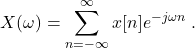
This is the known as the Discrete-time Fourier Transform.
Frequency Domain Periodicity
One of the important properties of the DTFT is that its frequency domain is periodic with a periodicity of  . That means that for every DTFT representation,

 . Typically, we study
 for frequencies in one period from
 to
 , where
 is the lowest frequency (before periodicity) and and are the highest negative and positive freqencies.
Show Proof
Consider the values of and  (where is an integer). This is defined by
(1) 
Since  and are integers, we know that
 . Therefore,
(2) 
This periodicity occurs because all discrete sine and cosine (and complex exponential, by extension) frequencies are always periodic with a period of .
Show Proof
Consider  . If we shift the frequency by
 (where is an integer), we get

Since and are both integers,  must a multiple of
 . A phase shift of any multiple of will not affect a sinusoid.
This property is also why the inverse DTFT is only integrated for a period of . This periodicity will be important to consider later since it affects how we design filters and plays a significant role in our discussion on signal resampling.
Existence
The DTFT of a discrete-time, aperiodic signal  is guaranteed to exist if

is a energy signal, it will satisfy this property.
Caveat: Some periodic signals (e.g., sines and cosines) can have a DTFT through the DTFT’s connection to the Discrete-Time Fourier Series and through the use of the Dirac delta function, even though periodic signals fail to satisfy the above property.
Difference Equations
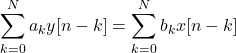
Discrete-time systems can be characterized by linear, constant-coefficient difference equations. That is a summation of shifted and weighted inputs will equal a summation of shifted and weighted outputs  such that
If we take the DTFT of both sides of this equation, we get that
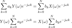
Hence, the transfer function becomes

Therefore, we can represent a system by difference equations.