One Filter, Many Forms: Why DSP Engineers Rebuild the Same Filter Over and Over Again

Disclaimer: this is an AI-generated article intended to highlight interesting concepts / methods / tools used within the Foundations of Digital Signal Processing course. This is for educating students as well as general readers interested in the course. The article may contain errors.

Direct form, cascade form, lattice form—filter structures aren’t just mathematical gimmicks. They’re your toolkit for making real-world systems stable, efficient, and actually work.

If you’re knee-deep in a graduate-level digital signal processing (DSP) course, you’ve probably designed a filter or two. You’ve plotted poles and zeros, wrangled a transfer function, maybe even written some MATLAB to test a low-pass filter on a noisy signal.

Then someone tells you:
“Great filter. Now pick your structure.”

Wait—what?

Isn’t a filter defined by its difference equation or transfer function? Isn’t that enough?

Short answer: no.

The long answer is what this article is about. Because when you move from the page to the real world—whether it’s a microcontroller, a medical device, or a machine learning pipeline—how you implement a filter matters just as much as what the filter does.

🎛️ A Filter Is More Than Its Transfer Function

Let’s take a typical IIR filter, described by the difference equation:

$y[n] = -a_1 y[n-1] - \cdots - a_N y[n-N] + b_0 x[n] + \cdots + b_M x[n-M]$

This corresponds to the transfer function:

$H(z) = \frac{b_0 + b_1 z^{-1} + \cdots + b_M z^{-M}}{1 + a_1 z^{-1} + \cdots + a_N z^{-N}}$

But this expression doesn’t tell you how to build it.

In implementation, we need to realize this as a structure—an actual diagram of multipliers, adders, and delays. This isn’t abstract: these structures define memory usage, roundoff behavior, and numerical stability. In real-time systems, especially those with fixed-point arithmetic, this can make or break your application.

Let’s walk through the most common filter structures, why they exist, and where they shine.

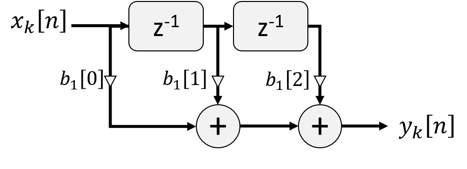
🧱 Direct Form I and II: The Textbook Workhorses

If you’ve ever hand-coded a filter from its difference equation, chances are you used Direct Form I.

It separates the feedforward (FIR) part and the feedback (IIR) part into two branches—one processing past inputs $x[n]$ , the other processing past outputs $y[n]$ .

Direct Form I Structure:

Requires $\max(M, N)$ delays for each branch.
Good conceptual mapping from the difference equation.
Common in high-level software (e.g., MATLAB’s filter()).

But Direct Form I uses twice as many delay elements as necessary.

Enter Direct Form II, which cleverly merges the delay lines using state-variable techniques:

Uses only $\max(M, N)$ delays in total.
More efficient in terms of memory.
But—more sensitive to roundoff error, especially in fixed-point systems.

So while Direct Form II is mathematically elegant, it’s not always the go-to in embedded applications.

🧩 Cascade Form: Divide and Conquer (Stability Edition)

Now here’s where things get interesting.

Suppose your IIR filter has a high-order denominator polynomial. In practice, implementing a single high-order filter is numerically risky. Small roundoff errors in the coefficients can shift poles, destroy stability, and wreck frequency response.

Solution? Break it up.

Using partial fraction expansion (or factoring polynomials), we express the transfer function as a product of second-order sections (SOS):

$H(z) = H_1(z) \cdot H_2(z) \cdot \cdots \cdot H_K(z)$

Each Hk(z)H_k(z)Hk(z) is a biquad—a second-order filter of the form:

$H_k(z) = \frac{b_0 + b_1 z^{-1} + b_2 z^{-2}}{1 + a_1 z^{-1} + a_2 z^{-2}}$

This is the cascade form. It has major benefits:

Improved numerical stability, especially in fixed-point.
Localizes errors to individual stages.
Allows modular tuning: change one section without rebuilding the entire system.
Well-suited for hardware and software libraries (e.g., ARM CMSIS DSP, SciPy’s sosfilt()).

If you’re designing a high-order filter for a hearing aid, seismic sensor, or biomedical device, cascade form is your friend.

🎚️ Parallel Form: When You Want Speed or Custom Gain Control

You can also expand a filter into parallel components using partial fraction expansion:

$H(z) = \sum_{k} \frac{A_k}{1 - p_k z^{-1}} + \text{(optional FIR term)}$

This parallel form is great when:

You want fine control over frequency bands.
You need fast dynamic range adjustments.
You’re implementing equalizers or reverberation units.

It’s less commonly hand-coded by students, but shows up a lot in audio plugins, where each resonant filter (e.g., shelving EQ) can be a separate path.

🪞 Lattice and Lattice-Ladder Structures: The Signal Processing Ninja Move

These aren’t usually the first structures you learn—but they’re important for adaptive filtering, speech processing, and systems that need robust numerical behavior.

The lattice structure represents a filter in terms of reflection coefficients, offering:

Excellent numerical stability.
Recursive design based on orthogonal polynomials.
Minimal roundoff sensitivity—even in real-time speech codecs.

If you’ve heard of Levinson-Durbin recursion, this is where it connects.

🛠️ Why So Many Structures?

Let’s pause and ask: why implement the same filter in so many different ways?

1. Numerical Stability

High-order polynomials are fragile. Small changes in coefficients can swing poles outside the unit circle, turning a stable system into an unstable one. Structures like cascade and lattice reduce this risk by working with smaller, well-behaved pieces.

2. Memory Constraints

In embedded systems—think wearables, IoT devices, or satellites—you might have only a few kilobytes of memory. Direct Form II uses fewer delay elements, making it more appealing than Direct Form I.

3. Hardware Optimization

Certain architectures (DSP chips, FPGAs, GPUs) have hardware pipelines optimized for biquad filters or in-place buffer reuse. Picking the right form lets you exploit this for real-time performance.

4. Modularity and Maintainability

Filter banks, EQs, and dynamic processors often rely on cascade or parallel forms to isolate bands or effects. This modularity makes tuning easier and more intuitive.

5. Application-Specific Constraints

Audio: Needs phase linearity and low noise—favor cascade and real-input optimizations.
Medical: Requires stability and power efficiency—favor lattice or direct form with careful scaling.
Radar/Comms: Needs fast reconfigurability—parallel or lattice forms often win here.

🎮 Analogy Time: Game Engines and Filter Structures

Think of filter structures like different game engines.

The game logic—your transfer function—is the same. But the rendering engine—how you implement and optimize—determines performance, responsiveness, and realism.

Want frame-perfect input? Use Unreal Engine. Want portability? Use Unity.
Want robust filters in a wearable ECG monitor? Use cascade form.
Want fast audio convolution on a GPU? Use a bank of FFT-based filters in parallel.

Same goals, different executions.

🧠 Final Thought: Choose Your Form with Purpose

Too often, filter design gets treated like a one-and-done operation: design, implement, done. But in professional DSP, the structure is not an afterthought—it’s part of the engineering solution.

Understanding the tradeoffs between forms helps you:

Build more efficient systems,
Prevent catastrophic bugs,
And collaborate across domains like hardware, software, and real-time signal processing.

So next time you’re handed a transfer function, don’t stop at the math. Ask the deeper question:

“What structure makes this filter work best in the real world?”

Because DSP isn’t just about transforming signals. It’s about transforming ideas into systems that work—with precision, speed, and clarity.

Filters Implementation Signal Processing

One Filter, Many Forms: Why DSP Engineers Rebuild the Same Filter Over and Over Again