Fast, Furious, and Fundamental: The Untold Depth of the Fast Fourier Transform

Disclaimer: this is an AI-generated article intended to highlight interesting concepts / methods / tools used within the Foundations of Digital Signal Processing course. This is for educating students as well as general readers interested in the course. The article may contain errors.

From music apps to quantum simulations, the FFT is the computational backbone of the modern world—and there’s more to it than radix-2 recursion.

We tend to treat algorithms as transient tools—clever bits of logic that solve specific problems and then fade into the background. But the Fast Fourier Transform, or FFT, is not that kind of algorithm.

The FFT isn’t just a fast way to compute a Fourier transform. It’s a cornerstone of digital signal processing, and by extension, of modern computation. It’s the engine beneath your voice assistant’s signal chain, the speed behind your MRI scanner’s image reconstruction, and the unsung hero of everything from wireless communication to deep learning.

Yet for many, the FFT begins and ends with a textbook diagram of a radix-2 butterfly. That’s a shame, because the FFT is both deeper and more diverse than its most famous form.

Let’s explore what the FFT really is, how it goes beyond radix-2, and why it remains one of the most influential ideas in the applied mathematical sciences.

🎧 The Core Idea: What the FFT Actually Computes

Let’s rewind for a second. The Discrete Fourier Transform (DFT) takes a sequence $x[n]$ , for $n = 0, 1, ..., N-1$ , and rewrites it in terms of complex exponentials:

$X[k] = \sum_{n=0}^{N-1} x[n] e^{-j \frac{2\pi}{N} kn}$

Each $X[k]$ represents how much of a frequency $\frac{k}{N}$ is present in the signal.

Naively computing the DFT takes $\mathcal{O}(N^2)$ operations. That’s fine for small signals—but for anything large, it’s a bottleneck.

The FFT, especially the radix-2 Cooley-Tukey algorithm, slashes this to $\mathcal{O}(N \log N)$ by recursively dividing the problem into smaller subproblems using the symmetry and periodicity of the exponential terms.

🌀 Radix-2 and the Butterfly Effect

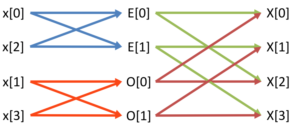
The most well-known FFT variant is the radix-2 decimation-in-time (DIT) algorithm. It works by splitting the input into even and odd-indexed samples and recursively applying the FFT:

$X[k] = E[k] + e^{-j \frac{2\pi}{N}k} \cdot O[k]$

Here, $E[k]$ and $O[k]$ are FFTs of the even and odd parts of $x[n]$ . This divide-and-conquer structure gives rise to the famous butterfly diagram, which visualizes how the data flows through the stages of computation.

This version works beautifully—as long as your data length $N$ is a power of 2.

But in practice, signals come in all shapes and sizes. So what happens when $N$ isn’t a power of 2?

🧠 Beyond Radix-2: Real-World FFTs Are Smarter

Radix-2 is only one member of a much larger family of FFT algorithms. Real-world applications often require more flexibility—and engineers have developed clever generalizations.

Mixed-Radix FFTs

When NNN has multiple prime factors (like $N = 60 = 2^2 \cdot 3 \cdot 5$ ), we can apply mixed-radix Cooley-Tukey algorithms. These break the DFT into stages based on each factor, using the same divide-and-conquer idea but with more variety in how the subproblems are handled.

This allows FFTs to handle nearly arbitrary lengths efficiently. You’ll find this in libraries like FFTW (“Fastest Fourier Transform in the West”), MATLAB’s fft(), Python’s SciPy, and even GPU-accelerated tools like cuFFT.

Prime Factor FFT (Good-Thomas Algorithm)

If the signal length is the product of relatively prime numbers (e.g., $N = 7 \cdot 11$ ), you can apply the Good-Thomas algorithm. This technique rearranges the input using the Chinese Remainder Theorem so the problem decouples nicely.

It’s less flexible than mixed-radix but useful in certain hardware implementations.

Bluestein’s Algorithm (Chirp-Z Transform)

For prime-length DFTs, Bluestein’s method transforms the DFT into a convolution, which is then computed efficiently using an FFT of larger size. It’s slower than radix-2 but often the only practical option for awkward lengths.

This flexibility is key in modern computation: real-world FFTs adapt to the input.

⚡ Hardware Optimization and Real-Input Tricks

Many real signals—like audio waveforms—are real-valued. That means their DFTs have conjugate symmetry:

$X[N - k] = X^*[k]$

Fast FFT libraries exploit this to halve the computation and memory usage. They also implement in-place algorithms that overwrite the input with the output to conserve space—essential in embedded and mobile systems.

Furthermore, FFTs are now optimized for parallelism. Libraries use SIMD instructions, multithreading, and GPU acceleration to deliver real-time performance on massive datasets. This is why FFTs power applications like:

Real-time spectral analysis
3D rendering
Signal compression
Wireless channel estimation
Audio synthesis and convolutional reverb

🧩 The DFT Isn’t Just Analysis—It’s Computation and Structure

Here’s something that students sometimes overlook: the DFT matrix is unitary. That means applying the DFT preserves energy, and its inverse is just the complex conjugate transpose, scaled:

$x[n] = \frac{1}{N} \sum_{k=0}^{N-1} X[k] e^{j \frac{2\pi}{N} kn}$

This unitarity is critical in applications like quantum computing, where transformations must conserve energy (or probability amplitude), and in numerical methods, where stability matters.

In short: the FFT isn’t just about speed. It’s about respecting structure.

🔁 Circular Convolution and Signal Processing

In DSP, the FFT’s most powerful use might be this:

Convolution in time becomes multiplication in frequency.

$x[n] * h[n] \xrightarrow{\text{FFT}} X[k] \cdot H[k]$

But here’s the twist: FFTs assume circular convolution, not linear. If your sequences aren’t periodic, this introduces time-domain aliasing. That’s why we zero-pad before taking the FFT:

$\text{If } \text{len}(x) = M, \text{len}(h) = L, \text{then pad both to } N \geq M + L - 1$

This trick allows fast convolution for filters, audio effects, and even image processing.

🌐 Modern Applications That Rely on FFTs

The FFT is not a niche algorithm—it’s in the DNA of modern computation:

AI and Deep Learning: FFTs are used to accelerate convolutions in neural networks (especially in resource-constrained settings).
Medical Imaging: MRI scanners reconstruct images by taking FFTs of radiofrequency signals in k-space.
Astronomy: Telescopes analyze signal spectra to identify distant stars and galaxies.
Finance: Quantitative analysts use FFTs for time-series prediction and anomaly detection.

And now, even physics-informed neural networks and graph Fourier transforms are extending FFT ideas to nonlinear and non-Euclidean domains.

🎬 Final Thought: The FFT Is Still Evolving

The Fast Fourier Transform is not a solved problem—it’s a living idea. From adaptive variants to quantum FFTs, researchers continue to push the boundaries of what’s possible. But its core insight remains timeless:

If you understand the structure of a problem, you can solve it faster, deeper, and more elegantly.

So whether you’re building a filter bank, analyzing brain waves, or reconstructing an image from incomplete data, the FFT isn’t just a function call. It’s a portal into the frequency domain, and a lesson in how mathematical beauty leads to real-world speed.

algorithms Fourier Transform Multi-rate Signal Processing

Fast, Furious, and Fundamental: The Untold Depth of the Fast Fourier Transform