Sampling – SmartDATA Lab

Sampling: Continuous-to-discrete

What is Sampling?

Sampling is the process of converting a continuous-time signal into a discrete time signal.

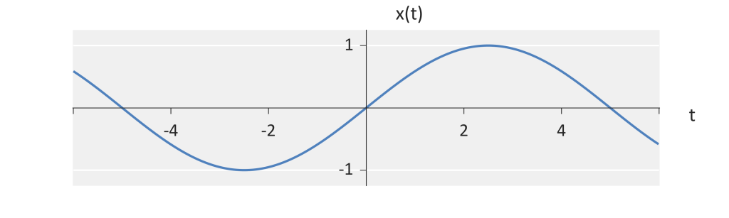
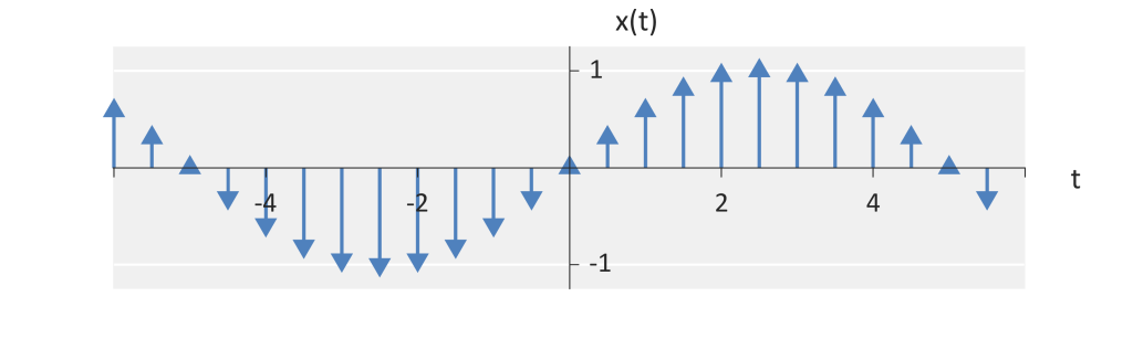
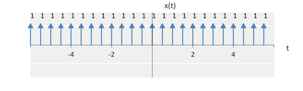
Sampling is accomplished by multiplying a continuous-time signal $x(t)$ with an impulse train, a periodic sequence of impulses with a fundamental period $T_s$ such that

$\delta_{T_s}(t) = \sum_{k=-\infty}^{\infty} \delta(t - k T_s) \; .$

We will use the notation $\delta_{T_s}(t)$ to represent a pulse train with sampling period $T_s$ . When we multiply $x(t)$ and $\delta_{T_s}(t)$ , we get an new train of impulses with amplitudes taken from $x(t)$ . Mathematically, we get

$x_s(t) = x(t) \delta_{T_s}(t) = \sum_{k=-\infty}^{\infty} x(k T_s) \delta(t - k T_s) \; .$

The question address in the rest of this class is: does the sampling process uniquely preserve all information about our signal?

Sampled sinusoid with sampling period of Ts=1.

Fourier Series/Transform of an impulse train

To answer this question, we look at the Fourier series/transform of the impulse train. Since $\delta_{T_s}(t)$ is periodic, we use the Fourier series. When we plug $\delta_{T_s}(t)$ into the Fourier analysis equation, we get

$c_k = \frac{1}{T_s} \int_{T_s} \delta_{T_s}(t) e^{-j k \Omega_s t} dt \; .$

Over one period, $\delta_{T_s}(t)$ is just an impulse. Therefore, the Fourier analysis equation simplifies to

$\begin{align*} c_k &=& \frac{1}{T_s} \int_{-T_s/2}^{T_s/2} \delta(t) e^{-j k \Omega_s t} dt \\ &=& \frac{1}{T_s} (1) \end{align*}$

We refer to $\Omega_s = 2 \pi / T_s$ as the [angular] sampling frequency.

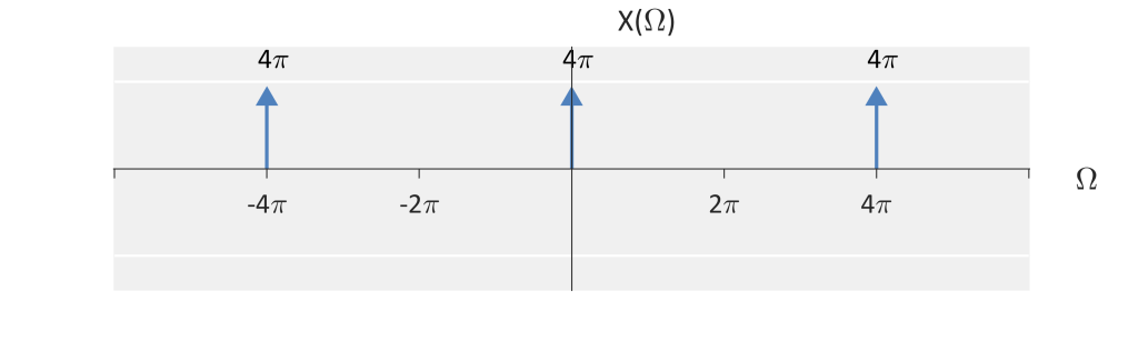
Since the Fourier series coefficients are defined by $c_k = \frac{1}{T_s}$ , the Fourier transform has a value of $2 \pi / T_{s}$ (the $2 \pi$ is introduced because we are in the angular frequency domain) at $k$ times the fundamental angular frequency, i.e. $k \Omega_s = k 2 \pi / T_s$ , where $k$ is an any integer. Therefore, in the continuous-frequency, we get a pulse train with spacing of $\Omega_s$ ,

$\begin{align*} \delta_{T_s}(t) &\stackrel{\mathcal{F}}{\longleftrightarrow}& \frac{2 \pi}{T_s} \delta_{\Omega_s}(\Omega) \\ \end{align*}$

Therefore, the Fourier transform of an infinite pulse train with period $T_s$ (i.e., $\delta_{T_s}(t))$ is a infinite pulse train with spacing $\Omega_s = 2 \pi / T_s$ (i.e., $({2 \pi}/{T_s}) \delta_{\Omega_s}(\Omega)$ ).

Fourier transform of the above pulse train.

Apply multiplication property

To determine the Fourier transform of $x(t) \delta_{T_s}(t)$ , we apply the multiplication property. That is, multiplication in time is equivalent to convolution in frequency. We get the relationship

$\begin{align*} x(t) \delta_{T_s}(t) &\stackrel{\mathcal{F}}{\longleftrightarrow}& \frac{1}{2 \pi} \left[ X(\Omega) * \left( \frac{2 \pi}{T_s} \delta_{\Omega_s}(\Omega) \right) \right] \\ x(t) \delta_{T_s}(t) &\stackrel{\mathcal{F}}{\longleftrightarrow}& \frac{1}{T_s} \sum_{k=-\infty}^{\infty} X(\Omega - k \Omega_s) \end{align*}$

Therefore, sampling in time results in the sum of shifted replicas of the frequency domain representation $X(\Omega)$ .

The Fourier transform of the above Gaussian pulse.

A sampled Gaussian pulse signal with sampling period of Ts=1/2 and sampling rate of Ωs=4π.

The Fourier transform the sampled Gaussian pulse with a sampling rate of Ωs=4π.

The sampling theorem

We can now answer our question, does the sampling process uniquely preserve all information about our signal? The answer is: yes, but under certain conditions.

Let the Fourier transform of $x(t)$ be $X(\Omega)$ with a largest angular frequency $\Omega_{max}$ . That is

$X(\Omega) = 0 \quad \textrm{for} \quad |\Omega| > \Omega_{max} \; .$

Also, let $X_{s}(\Omega)$ be defined as the Fourier transform of the sampled signal $x_s(t) = x(t) \delta_{T_s}(t)$ such that

$X_{s}(\Omega) = \frac{1}{T_s} \sum_{k=-\infty}^{\infty} X(\Omega - k \Omega_s) \; .$

If the bandwidth of the $X(\Omega)$ , $X(\Omega-\Omega_s)$ , and $X(\Omega+\Omega_s)$ never overlap, then the original frequency information is remains changed. That is, to preserve all information about the original signal, we require

$\Omega_s > 2 \Omega_{max}$

or, equivalently,

$\begin{align*} f_s &>& 2 f_{max} \\ T_s &<& \frac{1}{2 f_{max}} \\ T_s &<& \frac{\pi}{\Omega_{max}} \end{align*}$

Therefore, the sampling frequency, or sampling rate, must be two times larger than the maximum frequency in the signal. This is known as the sampling theorem or sampling criteria. The frequency $2 f_{max}$ or $2 \Omega_{max}$ is known as the Nyquist sampling rate.