Impulse Responses and Difference Equations

Convolution and Difference Equations

We previously demonstrated that the output of any linear, time-invariant system can be expressed by a convolution of an input and system impulse response. Here, we show that convolutions can be expressed with differences equations. Hence, any linear, time-invariant system can be expressed by difference equations.

The Difference Equation Form of Convolution

If we use the commutativity property (x[n] * h[n] = h[n] * x[n]), we see that the convolution can be written as

    \[y[n] = \sum_{m=-\infty}^{\infty} x[m] h[n - m] = \sum_{m=-\infty}^{\infty} h[m] x[n - m]\]

Hence, we can write this as:

    \[y[n] = \cdots + h[-2] x[n+2] + h[-1] x[n+1] + h[0] x[n-0] + h[1] x[n-1] + h[2] x[n-2] + \cdots\]

Since \ldots,h[-2],h[-1],h[0],\ldots are all constant values, the expression above is a difference equation.

Impulse Response Properties

Using our new definition, we can we can derive relationship between our impulse response h[n] and system properties.

Memoryless

An LTI system with impulse response h[n] is memoryless if

    \[h[n] = a \, \delta[n]\]

for any scalar constant a.

Causal / Anti-Causal

An LTI system with impulse response h[n] is causal if

    \[h[n] = 0 \qquad \textrm{for } n < 0\]

An LTI system with impulse response h[n] is anti-causal if

    \[h[n] = 0 \qquad \textrm{for } n \geq 0\]

A causal system must be dependent on only past and present values. As a difference equation, this can be written as

    \[y[n] = h[0] x[n-0] + h[1] x[n-1] + h[2] x[n-2] + \cdots\]

Hence, this is equivalent to stating h[n] = 0 for all n < 0:

    \[y[n] = \cdots + (0) x[n+2] + (0) x[n+1] + h[0] x[n-0] + h[1] x[n-1] + h[2] x[n-2] + \cdots\]

BIBO Stable

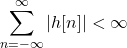
An LTI system with impulse response h[n] is BIBO stable if

    \[\sum_{n=-\infty}^{\infty} |h[n]| < \infty\]

Finite / Infinite Impulse Responses

FIR Filters

If the impulse response h[n] is finite in length (i.e., the number of non-zero values is finite), then the number of terms in the difference equation is finite. We refer to these types of linear, time-invariant systems as finite impulse response filters.

IIR Filters

If the impulse response h[n] is infinite in length, the linear, time-invariant systems is a infinite impulse response filter.

Relative to the difference equation, the impulse response h[n] may be infinite to two reasons.

The number of difference equation terms is infinite.

The difference equation has recursion (i.e., y[n] is a function of y[n-N] for any N)

When we have recursive terms, the difference equation can be written as

    \[\cdots + g[-2] y[n+2] + g[-1] y[n+1] + g[0] y[n-0] + g[1] y[n-1] + g[2] y[n-2] + \cdots \ = \ \cdots + h[-2] x[n+2] + h[-1] x[n+1] + h[0] x[n-0] + h[1] x[n-1] + h[2] x[n-2] + \cdots\]

This can be written as convolutions

    \[g[n] * y[n] = h[n] * x[n]\]

Hence, this is the general expression for relating any difference equation to convolutions.

Graphically understanding difference equations

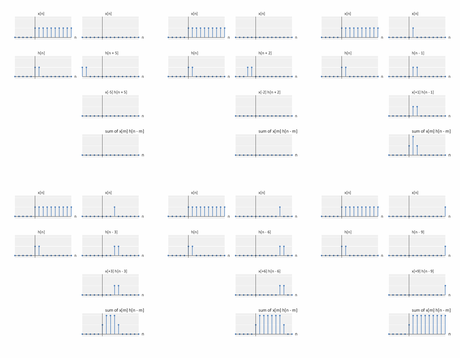
Convolution can be seen as a graphical process:

Plot x[n-m] with dependent variable n (m shifts the signal).

Plot h[n] with dependent variable n.

For each shift, compute h[m] x[n-m]. These are just weighted version of x[n-m].

Sum your elements to get y[n] = \sum_{m=-\infty}^{\infty} h[m] x[n-m].

Graphical Difference Equation Examples

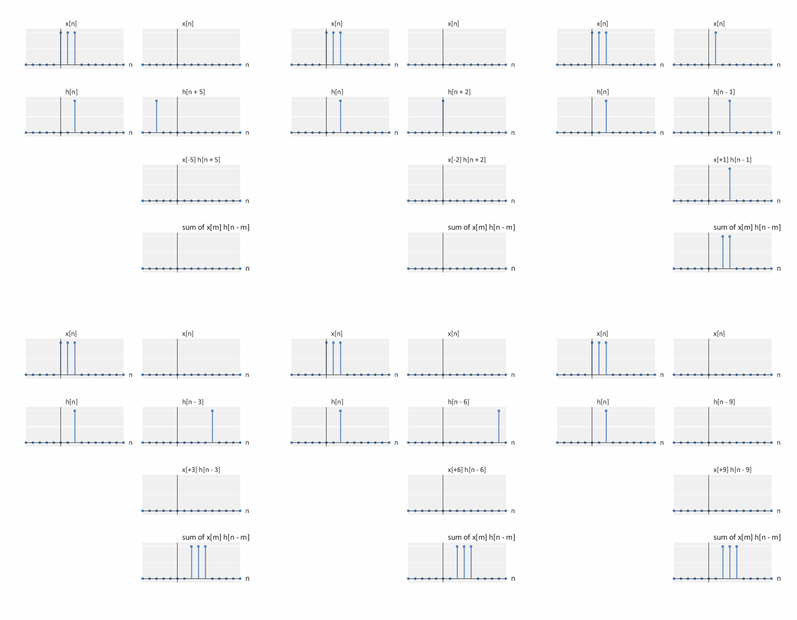
Below are a collection of graphical examples of discrete-time convolution / difference equation solutions.

Box and an impulse

x[n] = u[n] - u[n-3]
h[n] = \delta[n - 2]
y[n] = x[n] * h[n]

An animation of a convolution between a box and a shifted impulse (difference equations perspective)
An animation of a convolution between a box and a shifted impulse

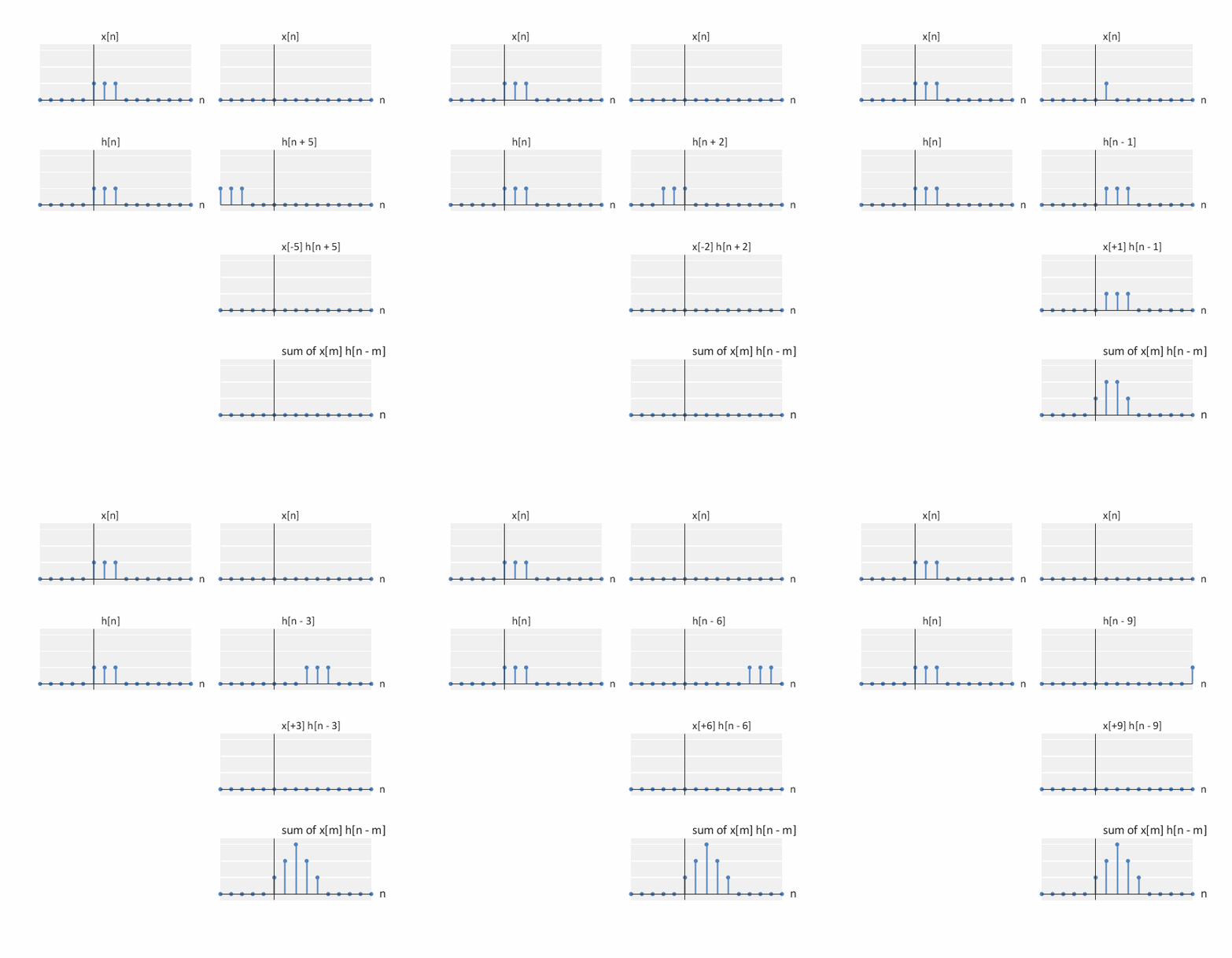
Two boxes

x[n] = u[n] - u[n-3]
h[n] = u[n] - u[n-3]
y[n] = x[n] * h[n]

An animation of a convolution between two boxes (difference equations perspective)
An animation of a convolution between two boxes

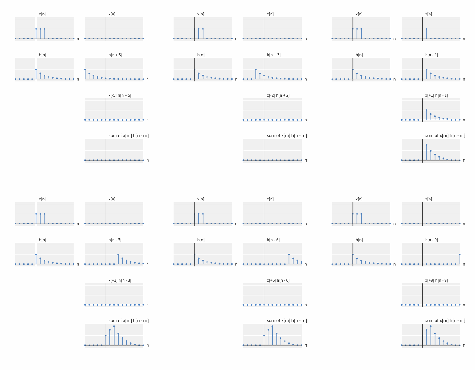
Box and exponential

x[n] = u[n] - u[n-3]
h[n] = e^{(-1/2) n} u[n]
y[n] = x[n] * h[n]

An animation of a convolution between a box and an exponential (difference equations perspective)
An animation of a convolution between a box and an exponential

Two exponentials

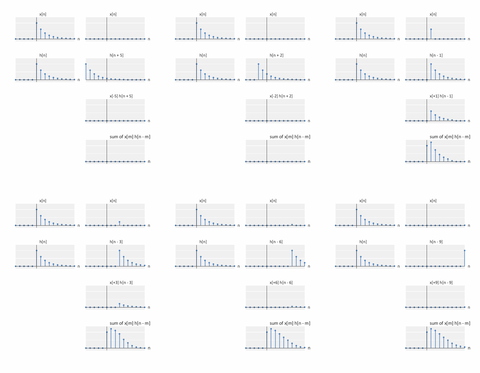
x[n] = e^{(-1/2) n} u[n]
h[n] = e^{(-1/2) n} u[n]
y[n] = x[n] * h[n]

An animation of a convolution between two exponentials (difference equations perspective)
An animation of a convolution between two exponentials

Finite Ramp and Box

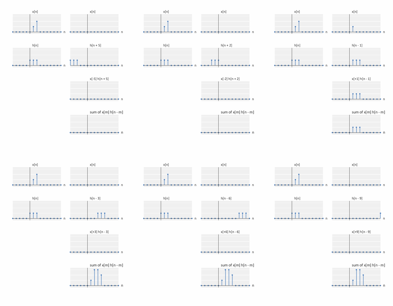
x[n] = \delta[n-1] + 2 \delta[n-2]
h[n] = u[n] - u[n-3]
y[n] = x[n] * h[n]

An animation of a convolution between a ramp and a box (difference equations perspective)
An animation of a convolution between a ramp and a box

Random Numbers and Box

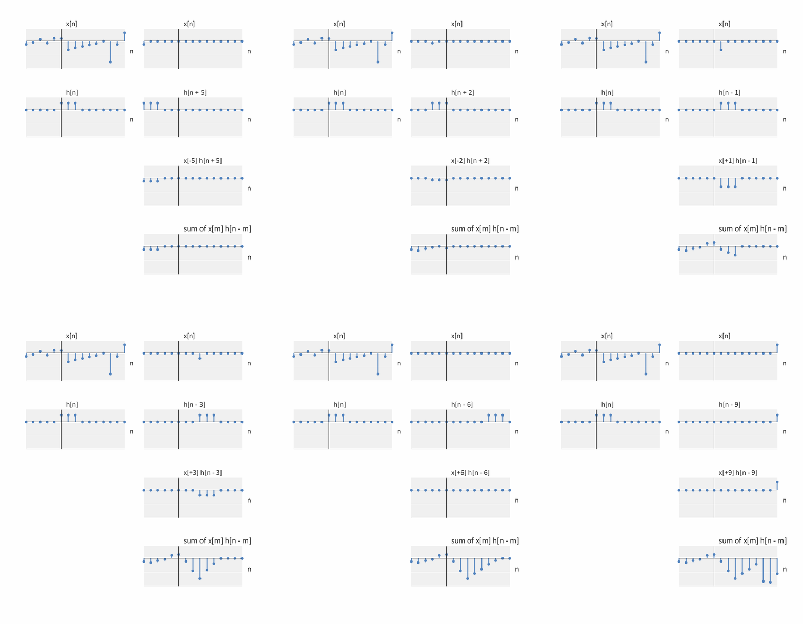
x[n] = random signal
h[n] = u[n] - u[n-3]
y[n] = x[n] * h[n]

An animation of a convolution between a random signal and a box (difference equations perspective)
An animation of a convolution between a random signal and a box

Step function and an exponential

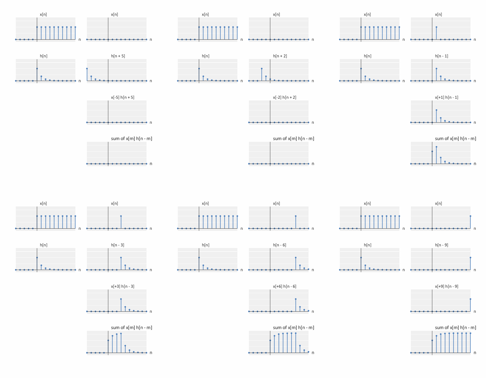
x[n] = u[n]
h[n] = e^{(-1/2) n} u[n]
y[n] = x[n] * h[n]

An animation of a convolution between a step and an exponential (difference equations perspective)
An animation of a convolution between a step and an exponential

Step function and a box

x[n] = u[n]
h[n] = u[n] - u[n-2]
y[n] = x[n] * h[n]

An animation of a convolution between a step and a box (difference equations perspective)
An animation of a convolution between a step and a box