Motivation
To analyze and process signals, we must first understand their basic properties: what types of signals exist, how we can measure their size, and how they respond to common operations like shifting and scaling. These properties provide the foundation for almost every concept in signal processing. Before we explore systems and transforms, we begin by precisely defining and classifying signals themselves.
Types of signals
Continuous / Discrete
A continuous-time signal x(t) is represented by an uncountably infinite number of dependent variable points (e.g., an uncountably infinite number of values across time).
A discrete-time signal x[n] is represented by a countable (potentially infinite, but not necessarily) number of dependent variable values (e.g., five values across time).
Notation warning: Some texts use the same bracket notation for both continuous-time and discrete-time signals (i.e., x(t) is continuous-time and x[n] is discrete-time). Furthermore, the book denotes discrete-time using m (common in controls literature) rather than n (common in signal processing literature). In this course, we will denote continuous-time signal with round brackets (⋅) and discrete-time signals by square brackets [⋅]. Further, we will typically use t to denote continuous-time signals and n to denote discrete-time signals. Note though that the dependent variable does not need to be time. It could be anything — time, space, speed, force, etc.


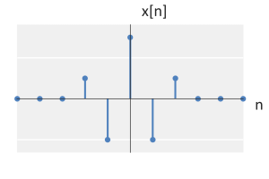
Even / Odd
The continuous-time signals x(t) is even when  .
The continuous-time signals x(t) is odd when  .
The discrete-time signals x[n] is even when  .
The discrete-time signals x[n] is odd when  .



Causal / Acausal
A continuous-time signal x(t) is said to be causal when

A continuous-time signal x(t) is said to be anticausal when

A discrete-time signal x[n] is said to be causal when

A discrete-time signal x[n] is said to be anticausal when

Signals that are not causal are also called acausal. Anticausal signals are a type acausal signals.


Periodic / Aperiodic
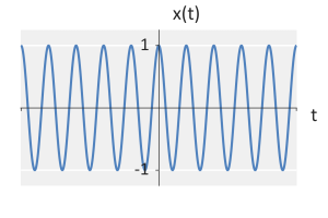
A continuous-time signal x(t) or discrete-time signal x[n] is said to be periodic if some  or
 exists such that

or is finite and  can equal any integer value. The smallest or that satisfies the above conditions is the fundamental period.
The fundamental cyclic frequency is the reciprocal of the fundamental period, such that  or
 . All other frequencies in the signal are defined by
 where m is any integer. These frequencies are known as harmonics.
The fundamental angular frequency is defined by  . Angular frequency is notationally convenient since the functions
 and
 will have angular frequencies of
 and
 , respectively.
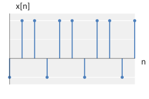
Caveat (discrete-time): Some signals that are periodic in continuous time are not periodic in discrete time. For example,  is not periodic because
 does not repeat with a rational multiple of
 .
Measures of signal “size”
Energy
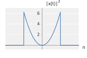
The energy of a continuous-time signal  is defined by

 is

 ).
Physical Interpretation: Energy, in this context, does not refer to a specific physical property. Instead, it describes the “size” of a signal. Our energy, however, can be related to electrical energy. If is a voltage signal across a load or resistance  , then the energy supplied to that load is
 .



Power (sometimes referred to as average power)
The power of a continuous-time signal is defined by


The power of a discrete-time signal is


 is a period of the periodic signal. This is equivalent to saying that the power of a periodic signal is equal to the average energy in one period of the signal.
A power signal is a signal with finite power (i.e.,  ).
Physical Interpretation: Power, in this context, does not refer to a specific physical property. Instead, it describes the “size” of a periodic signal. Our power, however, can be related to electrical power. If is a voltage signal across a load of resistance , then the power supplied to that load is  .
Important signal operations
Time shifting
The continuous-time signal  is the signal shifted to the right by
 units.
The continuous-time signal  is the signal shifted to the left by units.
The discrete-time signal  is the signal shifted to the right by samples.
The discrete-time signal  is the signal shifted to the left by samples.


Time scaling
Continuous time:
The continuous-time signal  is the signal x(t) condensed by a factor of
 .
The continuous-time signal  is the signal x(t) expanded by a factor of .
Discrete time:
Scaling only works when is an integer.
The discrete-time signal  is the signal x[n] downsampled by a factor of .
The discrete-time signal  is the signal x[n] upsampled (zero-insert) by a factor of .


Time reversal
The continuous-time signal  is the time-reversed signal of .
The discrete-time signal  is the time-reversed replica of signal .


Special functions / signals
Impulse functions
The Dirac δ signal (continuous-time impulse signal) is defined by

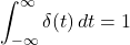
The Kronecker  signal (discrete-time impulse signal) is defined by

The properties of impulse signals:
- Energy:

- Power:

- Even / Odd?: Even (Understanding why is beyond the purview of this course. You will not be tested on this.)
- Periodic?: No
- Causal?: Yes


Heaviside step functions
The continuous-time Heaviside step function  is defined by

The discrete-time Heaviside step function  is defined by

The properties of the Heaviside step functions:
- Energy:

- Power:

- Even / Odd?: Neither
- Periodic?: No
- Causal?: Yes


Other Important Signals
Cosines and sines
The continuous-time cosine and sine signals are defined by

The properties of the continuous-time cosines or sines:
- Energy:

- Power:

- Even / Odd?:
 is even and
 is odd
- Periodic?: Yes
- Fundamental frequency:

- Fundamental period:

- Fundamental frequency:
- Causal?: No


Stepped exponential
A continuous-time exponential signal is defined by 
The properties of the exponential signals are:
- Energy:

- Power:

- Even / Odd?: No
- Periodic?: No
- Causal?: Yes

Complex exponentials
The continuous-time complex exponential signal is defined by 
The properties of the continuous-time complex exponential:
- Energy:
- Power:

- Even / Odd?: No, but its components are: cos(ω0t) is even and sin(ω0t) is odd
- Periodic?: Yes
- Fundamental frequency:
- Fundamental period:
- Fundamental frequency:
- Causal?: No

Stepped general exponential
The continuous-time general exponential signal is defined by 
The properties of the general exponential signals are:
- Energy:

- Power:
- Even / Odd?: No
- Periodic?: No
- Causal?: Yes
