Z-Transform – SmartDATA Lab

Motivation

We previously demonstrated that we can express any linear, time-invariant system with convolution or as difference equations. Yet, these representations can be challenging to work with, both theoretically and computationally. To address the theoretical complexity, we can transform signals into new representations that are easier to manipulate and interpret. The first transform we consider is the Z-transform.

The Z-transform excels at improving our understanding of the transient properties of signals. We will start to explore the Z-transform from a fairly theoretical perspective. As we go through the first half of the course, we will expand our conceptual understanding.

The Bilateral Z-Transform

Definition

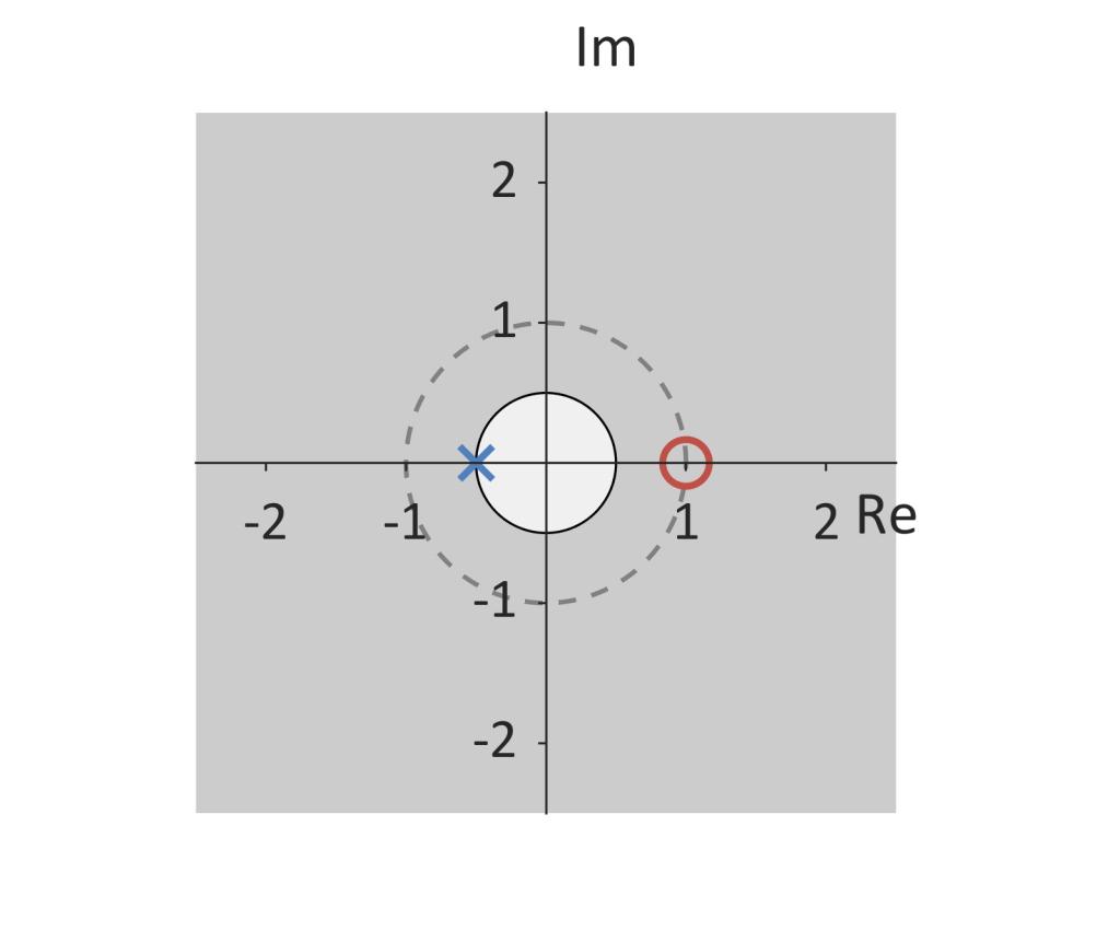
Causal region of convergence (dark grey area) for a system with a pole at z=−0.5 and a zero at z=1.

The bilateral Z-Transform and inverse Z-transform are defined by

$X(z) = \sum_{n=-\infty}^{\infty} x[n] z^{-n} \qquad , \qquad x[n] = \frac{1}{2 \pi j} \oint_{\mathcal{C}} X(z) z^{n-1} dz \; ,$

where $z$ is a complex number, $z = \sigma e^{j \omega}$ and $\mathcal{C}$ is a closed contour encircling the origin and lying entirely within the region of convergence (see below).

The unilateral Z-Transform and inverse Z-transform, used for causal signals ( $x[n] = 0$ when $n < 0$ ), is defined as

$X(z) = \sum_{n=0}^{\infty} x[n] z^{-n} \qquad , \qquad X(z) = \sum_{n=0}^{\infty} x[n] z^{-n} \; .$

Here, $z^{-n}$ represents a decaying complex exponential. The magnitude $\sigma$ controls the decay or growth rate, distinguishing the Z-transform from the DTFT (which uses $|z| = 1$ ).

Z-Transform and Difference Equations

A general linear, time-invariant system can be expressed as:

$\begin{align*}a[n] * y[n] &= b[n] * x[n] \\\sum_{m=-\infty}^{\infty} a[m] y[n-m] &= \sum_{m=-\infty}^{\infty} b[m] x[n-m] \; .\end{align*}$

In the Z-domain:

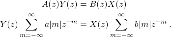
$\begin{align*} A(z) Y(z) &= B(z) X(z) \\ Y(z) \sum_{m=-\infty}^{\infty} a[m] z^{-m} &= X(z) \sum_{m=-\infty}^{\infty} b[m] z^{-m} \; . \end{align*}$

This leads to the transfer function:

$\begin{align*} H(z) &= \frac{Y(z)}{X(z)} = \frac{B(z)}{A(z)} \\ &= \frac{\sum_{m=-\infty}^{\infty} b[m] z^{-m}}{\sum_{m=-\infty}^{\infty} a[m] z^{-m}} \; . \end{align*}$

For a causal system with $M+1$ feedforward terms and $N+1$ feedback terms:

$\begin{align*} H(z) &= \frac{\sum_{m=0}^{M} b[m] z^{-m}}{\sum_{m=0}^{N} a[m] z^{-m}} \\ &= z^{-M+N} \frac{b_0}{a_0} \frac{\prod_{m=1}^{M} \left( z - z_{m} \right) }{\prod_{m=1}^{N} \left( z - p_{m} \right)} \\ &= \frac{b_0}{a_0} \frac{\prod_{m=1}^{M} \left( 1 - z_{m} z^{-1} \right) }{\prod_{m=1}^{N} \left( 1 - p_{m} z^{-1} \right)} \; , \end{align*}$

where $a_0 = a[0]$ and $b_0 = b[0]$ .

Show Proof

A linear time-invariant system can be represented by

$\cdots + a[-2] y[n+2] + a[-1] y[n+1] + a[0] y[n-0] + a[1] y[n-1] + a[2] y[n-2] + \cdots \\ = \\ \cdots + b[-2] x[n+2] + b[-1] x[n+1] + b[0] x[n-0] + b[1] x[n-1] + b[2] x[n-2] + \cdots$

If we take the Z-transform of this difference equation formulation, we get

$\cdots + a[-2] Y(z) z^2 + a[-1] Y(z) z^1 + a[0] Y(z) + a[1] Y(z) z^{-1} + a[2] Y(z) z^{-2} + \cdots \\ = \\ \cdots + b[-2] X(z) z^{2} + b[-1] X(z) z^{1} + b[0] X(z) + b[1] X(z) z^{-1} + b[2] X(z) z^{-2} + \cdots$

if we simplify this, we get

$Y(z) \left[ \cdots + a[-2] z^2 + a[-1] z^1 + a[0] + a[1] z^{-1} + a[2] z^{-2} + \cdots \right] \\ = \\ X(z) \left[ \cdots + b[-2] z^{2} + b[-1] z^{1} + b[0] + b[1] z^{-1} + b[2] z^{-2} + \cdots \right]$

$Y(z) \left[ \sum_{m=-\infty}^{\infty} a[m] z^{-m} \right] = X(z) \left[ \sum_{m=-\infty}^{\infty} b[m] z^{-m} \right]$

We can rearrange this equation to get

$H(z) = \frac{Y(z)}{X(z)} = \frac{\sum_{m=-\infty}^{\infty} b[m] z^{-m}}{\sum_{m=-\infty}^{\infty} a[m] z^{-m}} \; .$

Hence, the numerator and denominators are polynomials of $z^{-1}$ . If the system is causal, only $z^{-m}$ for $m \geq 0$ remain, resulting in

$H(z) = \frac{Y(z)}{X(z)} = \frac{\sum_{m=0}^{\infty} b[m] z^{-m}}{\sum_{m=0}^{\infty} a[m] z^{-m}} \; .$

The numerator and denominator of this expression are polynomials in $z^{-1}$ . We can make this a polynomials of $z$

$\begin{align*} H(z) &= \frac{b[0] z^{-M}}{a[0] z^{-N}} \frac{\sum_{m=0}^{M} (b[m]/b[0]) z^{m}}{\sum_{m=0}^{N} (a[m]/a[0]) z^{m}} \end{align*}$

and a polynomial with $M$ or $N$ terms can be factored into $M-1$ or $N-1$ terms

$\begin{align*} H(z) &= \frac{b[0] z^{-M}}{a[0] z^{-N}} \frac{\prod_{m=1}^{M} \left( z - z_{m} \right) }{\prod_{m=1}^{N} \left( z - p_{m} \right)} \\ &= \frac{b[0]}{a[0]} \frac{\prod_{m=1}^{M} \left( 1 - z_{m} z^{-1} \right) }{\prod_{m=1}^{N} \left( 1 - p_{m} z^{-1} \right)} \end{align*}$

The ratio of $Y(z)$ to $X(z)$ is known at the transfer function of the system.

Poles and Zeros

From the form

$H(z) = \frac{b_0}{a_0} \frac{\prod_{m=1}^{M} \left( 1 - z_{m} z^{-1} \right) }{\prod_{m=1}^{N} \left( 1 - p_{m} z^{-1} \right)} \; ,$

the values $z_{m}$ are the zeros of $H(z)$ the values of $z$ such that $H(z) = 0$ . The values $p_{m}$ are the poles values of $z$ such that $H(z) = \infty$ . Here, $M$ is the order of the numerator polynomial, and $N$ is the order of the denominator polynomial. Poles and zeros are typically plotted in the complex plane (real vs. imaginary axes).

The $z_{m}$ values are the zeros of $H(z)$ (i.e., the values of $z$ such that $H(z) = 0$ ). The $p_{m}$ values are the poles of $H(z)$ (i.e., the values of $z$ such that $H(z) = \infty$ ).

The figures below illustrate how we plot poles and zeros in the complex (real-imaginary) plane.

Z-Transform Pairs

$\begin{align*} \hline & x[n] &\qquad & X(z) &\qquad & \textrm{Region of Convergence} \\ \hline & \displaystyle a^n u[n] &\qquad & \displaystyle \frac{1}{1 - a z^{-1}} &\qquad & |z| > |a| \\ & \displaystyle - a^n u[- n - 1] &\qquad & \displaystyle \frac{1}{1 - a z^{-1}} &\qquad & |z| < |a| \\ & \displaystyle n a^n u[n] &\qquad & \displaystyle \frac{a z^{-1}}{(1-a z^{-1})^2}&\qquad & |z| > |a| \\ & \displaystyle - n a^n u[-n - 1] &\qquad & \displaystyle \frac{a z^{-1}}{(1-a z^{-1})^2}&\qquad & |z| < |a| \\ & \displaystyle \delta[n] &\qquad & \displaystyle 1 &\qquad & \textrm{All } z \\ & \displaystyle \delta[n - n_0] &\qquad & \displaystyle z^{-n_0} &\qquad & \textrm{All } z \\ & \displaystyle u[n] &\qquad & \displaystyle \frac{1}{1 - z^{-1}}&\qquad & |z| > 1 \\ & \displaystyle \cos(\omega_0 n) u[n] &\qquad & \displaystyle \frac{ 1 - z^{-1} \cos(\omega_0) }{1 - 2 z^{-1}\cos(\omega_0) + z^{-2} } &\qquad & |z| > 1 \\ & \displaystyle \sin(\omega_0 n) u[n] &\qquad & \displaystyle \frac{ z^{-1} \sin(\omega_0) }{1 - 2 z^{-1}\cos(\omega_0) + z^{-2} } &\qquad & |z| > 1 \\ & \displaystyle a^n \cos(\omega_0 n) u[n] &\qquad & \displaystyle \frac{ 1 - a z^{-1} \cos(\omega_0) }{1 - 2 a z^{-1}\cos(\omega_0) + a^2 z^{-2} } &\qquad & |z| > |a| \\ & \displaystyle a^n \sin(\omega_0 n) u[n] &\qquad & \displaystyle \frac{ a z^{-1} \sin(\omega_0) }{1 - 2 a z^{-1}\cos(\omega_0) + a^2 z^{-2} } &\qquad & |z| > |a| \\ \hline \end{align*}$

Z-Transform Properties

For each property, assume:

$x[n] \stackrel{Z}{\longleftrightarrow} X(z) \quad \textrm{and} \quad y[n] \stackrel{Z}{\longleftrightarrow} Y(z)$

$\begin{align*} \hline & \textbf{Property} &\qquad & \textbf{Time domain} &\qquad & \textbf{Z-domain} &\qquad \\ \hline & \textrm{Linearity} &\qquad & A x[n] + B y[n] &\qquad & A X(z) + B Y(z) &\qquad \\ & \textrm{Time Shifting} &\qquad & x[n-n_0] &\qquad & X(z)z^{-n_0} &\qquad \\ & \textrm{Z-scaling} &\qquad & a^n x[n] &\qquad & X(a^{-1} z) &\qquad \\ & \textrm{Conjugation} &\qquad & x^[n] &\qquad & X^(z^) &\qquad \\ & \textrm{Time Reversal} &\qquad & x[-n] &\qquad & X(z^{-1}) &\qquad \\& \textrm{Convolution} &\qquad & x[n] * y[n] &\qquad & X(z) Y(z) &\qquad \\ & \textrm{Differentiation in z-domain} &\qquad & n x[n] &\qquad & -z \frac{d X(z)}{d z} &\qquad \\ & \textrm{Initial Value Theorem} &\qquad & x[n] \textrm{ is causal} &\qquad & x(0) = \lim_{z \rightarrow \infty} X(z) &\qquad \\ & \textrm{Final Value Theorem} &\qquad & x[n] \textrm{ is causal and stable} &\qquad & x(\infty) = \lim_{z \rightarrow 1} [z-1] X(z) &\qquad \end{align*}$